How To Activate Your Free Office 2007 to 2010 Tech Guarantee Upgrade

Have you purchased Office 2007 since March 5th, 2010?  If so, here’s how you can activate and download your free upgrade to Office 2010!

Microsoft Office 2010 has just been released, and today you can purchase upgrades from most retail stores or directly from Microsoft via download.  But if you’ve purchased a new copy of Office 2007 or a new computer that came with Office 2007 since March 5th, 2010, then you’re entitled to an absolutely free upgrade to Office 2010.  You’ll need enter information about your Office 2007 and then download the upgrade, so we’ll step you through the process.

Getting Started

First, if you’ve recently purchased Office 2007 but haven’t installed it, you’ll need to go ahead and install it before you can get your free Office 2010 upgrade.  Install it as normal.

 

Once Office 2007 is installed, run any of the Office programs.  You’ll be prompted to activate Office.  Make sure you’re connected to the internet, and then click Next to activate.

Get your Free Upgrade to Office 2010

Now you’re ready to download your upgrade to Office 2010.  Head to the Office Tech Guarantee site (link below), and click Upgrade now.

You’ll need to enter some information about your Office 2007.  Check that you purchased your copy of Office 2007 after March 5th, select your computer manufacturer, and check that you agree to the terms.

Now you’re going to need the Product ID number from Office 2007.  To find this, open Word or any other Office 2007 application.  Click the Office Orb, and select Options on the bottom.

Select the Resources button on the left, and then click About.

Near the bottom of this dialog, you’ll see your Product ID.  This should be a number like:

12345-123-1234567-12345

 

Go back to the Office Tech Guarantee signup page in your browser, and enter this Product ID.  Select the language of your edition of Office 2007, enter the verification code, and then click Submit.

It may take a few moments to validate your Product ID.

When it is finished, you’ll be taken to an order page that shows the edition of Office 2010 you’re eligible to receive.  The upgrade download is free, but if you’d like to purchase a backup DVD of Office 2010, you can add it to your order for $13.99.  Otherwise, simply click Continue to accept.

Do note that the edition of Office 2010 you receive may be different that the edition of Office 2007 you purchased, as the number of editions has been streamlined in the Office 2010 release.  Here’s a chart you can check to see what edition you’ll receive.  Note that you’ll still be allowed to install Office on the same number of computers; for example, Office 2007 Home and Student allows you to install it on up to 3 computers in the same house, and your Office 2010 upgrade will allow the same.

Office 2007 Edition	Office 2010 Upgrade You’ll Receive
Office 2007 Home and Student	Office Home and Student 2010
Office Basic 2007 Office Standard 2007	Office Home and Business 2010
Office Small Business 2007 Office Professional 2007 Office Ultimate 2007	Office Professional 2010
Office Professional 2007 Academic Office Ultimate 2007 Academic	Office Professional Academic 2010

Sign in with your Windows Live ID, or create a new one if you don’t already have one.

Enter your name, select your country, and click Create My Account.  Note that Office will send Office 2010 tips to your email address; if you don’t wish to receive them, you can unsubscribe from the emails later.

 

Finally, you’re ready to download Office 2010!  Click the Download Now link to start downloading Office 2010.  Your Product Key will appear directly above the Download link, so you can copy it and then paste it in the installer when your download is finished.  You will additionally receive an email with the download links and product key, so if your download fails you can always restart it from that link.

If your edition of Office 2007 included the Office Business Contact Manager, you will be able to download it from the second Download link.  And, of course, even if you didn’t order a backup DVD, you can always burn the installers to a DVD for a backup.

 

Install Office 2010

Once you’re finished downloading Office 2010, run the installer to get it installed on your computer.  Enter your Product Key from the Tech Guarantee website as above, and clickContinue.

Accept the license agreement, and then click Upgrade to upgrade to the latest version of Office.

 

The installer will remove all of your Office 2007 applications, and then install their 2010 counterparts.  If you wish to keep some of your Office 2007 applications instead, clickCustomize and then select to either keep all previous versions or simply keep specific applications.

By default, Office 2010 will try to activate online automatically.  If it doesn’t activate during the install, you’ll need to activate it when you first run any of the Office 2010 apps.

 

Conclusion

The Tech Guarantee makes it easy to get the latest version of Office if you recently purchased Office 2007.  The Tech Guarantee program is open through the end of September, so make sure to grab your upgrade during this time.  Actually, if you find a great deal on Office 2007 from a major retailer between now and then, you could also take advantage of this program to get Office 2010 cheaper.

And if you need help getting started with Office 2010, check out our articles that can help you get situated in your new version of Office!

Getting Started With Microsoft Project 2010

Would you like to keep your projects on track and keep track of how time and resources are used?  Let’s take a look at Microsoft Project 2010 and how it can help you stay on top of your projects.

Microsoft Project 2010 is the latest version of Project, a companion project management application for Microsoft Office.  This version includes a wide range of changes, including the new ribbon interface.  Microsoft Project integrates with all the other Office application you regularly use,

Setting Up Project 2010

First, you’ll need to install Project 2010 on your computer.  If you haven’t purchased Project, you can try out a free 60 day trial from the link below.  The installer works just like the Office 2010 installer, so if you’ve already installed Office 2010 you’ll know what to expect.  Enter your product key to get started, then install as normal.

Microsoft Project will show up in your Start menu along with other Office applications you may have installed.

Now you’re ready to get started managing your projects in Microsoft Project 2010.

Manage Your Projects in Microsoft Project

When you first start Project, you’ll notice that it’s immediately ready for you to start entering tasks.  Simply enter a task name, duration, start and finish times, and any other details you need.  Your new tasks will show up automatically in the Gantt chart on the right, where you can drag the tasks to change the start and finish times.

You can make an existing tasks a sub-task easily.  Once you’ve entered the sub-task, simply hover over the task and your mouse will turn into an arrow.  Now drag the bar right or left to make the task a sub-task or remove it from being a sub-task.

It includes a wide variety of fields you can add to tasks so you can keep track of all important aspects.  Choose the things most important for this project.

Microsoft Project is designed to help you manage the whole team’s time, so you’ll want to add Resources, or the people involved in the project, to your new project.  You can quickly add new people to the project by entering their names in the Resource field.  Once you’ve entered different team members on various tasks, you’ll be able to select one from the drop-down menu.

Now, select the Resources tab on the top ribbon, and click the Details button.  This will open a details pane about your resources, where you can add the individual’s rate per hour, available time to work on the project, and more.

The Resource tab also lets you add resources, including material and cost resources.  You can also import people into your project from your Active Directory or Address Book.

Once you’ve added everyone’s rates and available times, you may notice some conflicts highlighted in red on your tasks.  Right-click on the task to see some solutions, or selectFix in Task Inspector to get more insight on how to solve the problems.

The Task Inspector helps you see what conflicts the employee or other resource may have, and will give you options to extend the deadline, add more people on the task, and more.  These features can help you manage your company without accidently overscheduling anyone.

As your projects grow more complex, you may find a different way to view your project would be helpful.  Simply click the chart button on the far left of the ribbon, and select from the wide range of built-in views, sheets, and reports you can use for your project.

Large projects can become unwieldy on their own, so at some point, you’ll need to decide to split tasks into new projects.  Microsoft Project lets you keep everything together, still, even if you need to move it into a new project file.  From the Project tab, you can link various projects together or create a subproject to keep everything in order.

You can also fully customize how your project looks from the ribbon, complete with various graphics styles for your Gantt charts.

Project offers a wide range of reports you can generate about your projects, including costs, workload, and more.  Note that you’ll have to enter all the available information in your tasks to make sure your reports are as accurate as possible.

Then, you can share your project details with your team in PDF format so everyone can use it whether they have Project or not.

Learning More About Project

Project can make it easier to manage your projects, but it can appear daunting at first.  Thankfully, Microsoft offers several resources that can help you get up to speed quickly and easily.  First, the built-in Help app contains some great information into how to put project management tools to use, including some basics of how project management itself works.

Then, you can download a quick reference guide (link below) that contains detailed steps to help you make useful Project files to make you and your team more efficient.

There are additionally many Project templates you can quickly download and look at to help you get a feel for how you can put Project to use.  Simply open the File tab, select New, then browse the available Office.com templates.  You’ll generally make the best plans for your own projects if you create your own new Project files, but these can give you ideas and let you see how you might break your project down into useful parts.

These resources should help you manage your projects better than ever in Project 2010.  Microsoft Project includes many features designed to help you efficiently manage your whole team’s time.  If you take the time to setup up tasks and plan appropriately, it can be a great help at planning new appointments and keeping everyone productive.

Learn More About Microsoft Project 2010

Download a free 60 day trial of Project Professional 2010

Download a Quick Reference Guide to get started with Project easily

How to Highlight a Row in Excel Using Conditional Formatting

Conditional formatting is an Excel feature you can use when you want to format cells based on their content. For example, you can have a cell turn red when it contains a number lower than 100. But how do you highlight an entire row?

If you’ve never used Conditional Formatting before, you might want to look at Using Conditional Cell Formatting in Excel 2007. It’s one version back, but the interface really hasn’t changed much.

But what if you wanted to highlight other cells based on a cell’s value? The screenshot above shows some codenames used for Ubuntu distributions. One of these is made up; when I entered “No” in the “Really” column, the entire row got different background and font colors. To see how this was done, read on.

Creating Your Table

The first thing you will need is a simple table containing the data you’d like to format. The data doesn’t have to be text-only; you can use formulas freely. At this point, your table has no formatting at all:

Setting The Look-and-Feel

Now it’s time to format your table using Excel’s “simple” formatting tools. Format only those parts that won’t be affected by conditional formatting. In our case, we can safely set a border for the table, as well as format the header line. I’m going to assume you know how to do this part. You should end up with a table looking like this (or maybe a bit prettier):

Creating The Conditional Formatting Rules

And now we come to the meat and potatoes. As we said at the outset, if you’ve never used conditional formatting before, this might be a tad too much to begin with. Read and try our earlier primer on the subject and once you’ve got that down, come back here. If you’re familiar with conditional formatting, let’s forge on.

Select the first cell in the first row you’d like to format, click Conditional Formatting (in the Home tab) and select Manage Rules.

In the Conditional Formatting Rules Manager click New Rule.

In the New Formatting Rule dialog, click the last option – Use a formula to determine which cells to format. This is the trickiest part: Your formula must evaluate to “True” for the rule to apply, and must be flexible enough so you could use it across your entire table later on. Let’s analyze my sample formula:

=$G15 – this part is a cell’s address. G is the column which I want to format by (“Really?”). 15 is my current row. Note the dollar sign before the G – if I don’t have this symbol, when I apply my conditional formatting to the next cell, it would expect  H15 to say “Yes”. So in this case, I need to have a “fixed” column ($G) but a “flexible” row (15), because I will be applying this formula across multiple rows.

=”Yes” – this part is the condition that has to be met. In this case we’re going for the simplest condition possible – it just has to say “Yes”. You can get very fancy with this part.

So in English, our formula is true whenever cell G in the current row has the word Yes in it.

Next, let’s define the formatting. Click the Format button. In the Format Cells dialog, go through the tabs and tweak the settings until you get the look you want.  Here we’ll just be changing the fill to a different color.

Once you’re got the desired look, click OK. You can now see a preview of your cell in the New Formatting Rule dialog.

Click OK again to get back to the Conditional Formatting Rules Manager and click Apply. If the cell you selected changes formatting, that means your formula was correct. If the formatting doesn’t change, you need to go a few steps back and tweak your formula until it does work.

Now that we have a working formula, let’s apply it across our entire table. As you can see above, the formatting applies only to the cell we started off with. Click the button next to the Applies to field and drag the selection across your entire table.

Once done, click the button next to the address field to get back to the full dialog. You should still see a marquee around your entire table, and now the Applies to field contains a range of cells and not just a single address. Click Apply.

Every row in your table should now be formatted according to the new rule:

That’s it! Now all you have to do is create another rule to format rows that say “No” (there was never an Ubuntu version called Chipper Chameleon, and we think that’s a shame). If your data is more complex, you may need to set up even more rules. Follow this method and in no time you’ll be creating intricate spreadsheets with data that pops right off the screen. Feel free to post screenshots of your creations in the comments!

Using VLOOKUP in Excel

VLOOKUP is one of Excel’s most useful functions, and it’s also one of the least understood.  In this article, we demystify VLOOKUP by way of a real-life example.  We’ll create a usable Invoice Template for a fictitious company.

So what is VLOOKUP?  Well, of course it’s an Excel function.  This article will assume that the reader already has a passing understanding of Excel functions, and can use basic functions such as SUM, AVERAGE, and TODAY.  In its most common usage, VLOOKUP is adatabase function, meaning that it works with database tables – or more simply, lists of things in an Excel worksheet.  What sort of things?   Well, any sort of thing.  You may have a worksheet that contains a list of employees, or products, or customers, or CDs in your CD collection, or stars in the night sky.  It doesn’t really matter.

Here’s an example of a list, or database.  In this case it’s a list of products that our fictitious company sells:

Usually lists like this have some sort of unique identifier for each item in the list.  In this case, the unique identifier is in the “Item Code” column.  Note:  For the VLOOKUP function to work with a database/list, that list must have a column containing the unique identifier (or “key”, or “ID”), and that column must be the first column in the table.  Our sample database above satisfies this criterion.

The hardest part of using VLOOKUP is understanding exactly what it’s for.  So let’s see if we can get that clear first:

VLOOKUP retrieves information from a database/list based on a supplied instance of the unique identifier.

Put another way, if you put the VLOOKUP function into a cell and pass it one of the unique identifiers from your database, it will return you one of the pieces of information associated with that unique identifier.  In the example above, you would pass VLOOKUP an item code, and it would return to you either the corresponding item’s description, its price, or its availability (its “In stock” quantity).  Which of these pieces of information will it pass you back?  Well, you get to decide this when you’re creating the formula.

If all you need is one piece of information from the database, it would be a lot of trouble to go to to construct a formula with a VLOOKUP function in it.  Typically you would use this sort of functionality in a reusable spreadsheet, such as a template.  Each time someone enters a valid item code, the system would retrieve all the necessary information about the corresponding item.

Let’s create an example of this:  An Invoice Template that we can reuse over and over in our fictitious company.

First we start Excel…

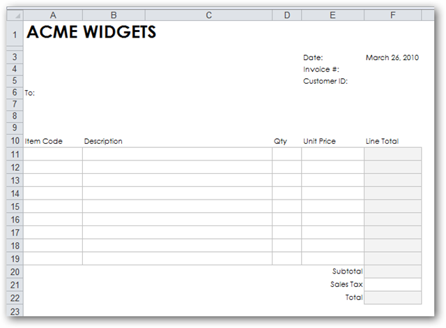
…and we create ourselves a blank invoice:

This is how it’s going to work:  The person using the invoice template will fill in a series of item codes in column “A”, and the system will retrieve each item’s description and price, which will be used to calculate the line total for each item (assuming we enter a valid quantity).

For the purposes of keeping this example simple, we will locate the product database on a separate sheet in the same workbook:

In reality, it’s more likely that the product database would be located in a separate workbook.  It makes little difference to the VLOOKUP function, which doesn’t really care if the database is located on the same sheet, a different sheet, or a completely different workbook.

In order to test the VLOOKUP formula we’re about to write, we first enter a valid item code into cell A11:

Next, we move the active cell to the cell in which we want information retrieved from the database by VLOOKUP to be stored.  Interestingly, this is the step that most people get wrong.  To explain further:  We are about to create a VLOOKUP formula that will retrieve the description that corresponds to the item code in cell A11.  Where do we want this description put when we get it?  In cell B11, of course.  So that’s where we write the VLOOKUP formula – in cell B11.

Select cell B11:

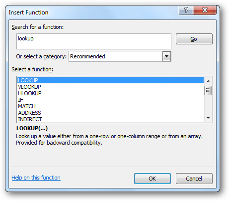
We need to locate the list of all available functions that Excel has to offer, so that we can choose VLOOKUP and get some assistance in completing the formula.  This is found by first clicking the Formulas tab, and then clicking Insert Function:

A box appears that allows us to select any of the functions available in Excel.  To find the one we’re looking for, we could type a search term like “lookup” (because the function we’re interested in is a lookup function).  The system would return us a list of all lookup-related functions in Excel.  VLOOKUP is the second one in the list.  Select it an click OK…

The Function Arguments box appears, prompting us for all the arguments (orparameters) needed in order to complete the VLOOKUP function.  You can think of this box as the function is asking us the following questions:

1. What unique identifier are you looking up in the database?
2. Where is the database?
3. Which piece of information from the database, associated with the unique identifier, do you wish to have retrieved for you?

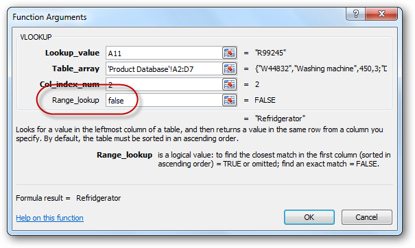
The first three arguments are shown in bold, indicating that they are mandatoryarguments (the VLOOKUP function is incomplete without them and will not return a valid value).  The fourth argument is not bold, meaning that it’s optional:

 

We will complete the arguments in order, top to bottom.

The first argument we need to complete is the Lookup_value argument.  The function needs us to tell it where to find the unique identifier (the item code in this case) that it should be retuning the description of.  We must select the item code we entered earlier (in A11).

Click on the selector icon to the right of the first argument:

Then click once on the cell containing the item code (A11), and press Enter:

The value of “A11” is inserted into the first argument.

Now we need to enter a value for the Table_array argument.  In other words, we need to tell VLOOKUP where to find the database/list.  Click on the selector icon next to the second argument:

Now locate the database/list and select the entire list – not including the header line.  The database is located on a separate worksheet, so we first click on that worksheet tab:

Next we select the entire database, not including the header line:

…and press Enter.  The range of cells that represents the database (in this case “’Product Database’!A2:D7”) is entered automatically for us into the second argument.

Now we need to enter the third argument, Col_index_num.  We use this argument to specify to VLOOKUP which piece of information from the database, associate with our item code in A11, we wish to have returned to us.  In this particular example, we wish to have the item’s description returned to us.  If you look on the database worksheet, you’ll notice that the “Description” column is the second column in the database.  This means that we must enter a value of “2” into the Col_index_num box:

It is important to note that that we are not entering a “2” here because the “Description” column is in the B column on that worksheet.  If the database happened to start in columnK of the worksheet, we would still enter a “2” in this field.

Finally, we need to decide whether to enter a value into the final VLOOKUP argument,Range_lookup.  This argument requires either a true or false value, or it should be left blank.  When using VLOOKUP with databases (as is true 90% of the time), then the way to decide what to put in this argument can be thought of as follows:

If the first column of the database (the column that contains the unique identifiers) is sorted alphabetically/numerically in ascending order, then it’s possible to enter a value oftrue into this argument, or leave it blank.

If the first column of the database is not sorted, or it’s sorted in descending order, then you must enter a value of false into this argument

As the first column of our database is not sorted, we enter false into this argument:

That’s it!  We’ve entered all the information required for VLOOKUP to return the value we need.  Click the OK button and notice that the description corresponding to item code “R99245” has been correctly entered into cell B11:

The formula that was created for us looks like this:

If we enter a different item code into cell A11, we will begin to see the power of the VLOOKUP function:  The description cell changes to match the new item code:

We can perform a similar set of steps to get the item’s price returned into cell E11.  Note that the new formula must be created in cell E11.  The result will look like this:

…and the formula will look like this:

Note that the only difference between the two formulae is the third argument (Col_index_num) has changed from a “2” to a “3” (because we want data retrieved from the 3rd column in the database).

If we decided to buy 2 of these items, we would enter a “2” into cell D11.  We would then enter a simple formula into cell F11 to get the line total:

=D11*E11

…which looks like this…

Completing the Invoice Template

We’ve learned a lot about VLOOKUP so far.  In fact, we’ve learned all we’re going to learn in this article.  It’s important to note that VLOOKUP can be used in other circumstances besides databases.  This is less common, and may be covered in future How-To Geek articles.

Our invoice template is not yet complete.  In order to complete it, we would do the following:

1. We would remove the sample item code from cell A11 and the “2” from cell D11.  This will cause our newly created VLOOKUP formulae to display error messages:
   
   We can remedy this by judicious use of Excel’s IF() and ISBLANK() functions.  We change our formula from this…
         =VLOOKUP(A11,’Product Database’!A2:D7,2,FALSE)
   …to this…
         =IF(ISBLANK(A11),”",VLOOKUP(A11,’Product Database’!A2:D7,2,FALSE))
2. We would copy the formulas in cells B11, E11 and F11 down to the remainder of the item rows of the invoice.  Note that if we do this, the resulting formulas will no longer correctly refer to the database table.  We could fix this by changing the cell references for the database to absolute cell references.  Alternatively – and even better – we could create a range name for the entire product database (such as “Products”), and use this range name instead of the cell references.  The formula would change from this…
         =IF(ISBLANK(A11),”",VLOOKUP(A11,’Product Database’!A2:D7,2,FALSE))
   …to this…
         =IF(ISBLANK(A11),”",VLOOKUP(A11,Products,2,FALSE))
   …and then copy the formulas down to the rest of the invoice item rows.
3. We would probably “lock” the cells that contain our formulae (or rather unlock theother cells), and then protect the worksheet, in order to ensure that our carefully constructed formulae are not accidentally overwritten when someone comes to fill in the invoice.
4. We would save the file as a template, so that it could be reused by everyone in our company

If we were feeling really clever, we would create a database of all our customers in another worksheet, and then use the customer ID entered in cell F5 to automatically fill in the customer’s name and address in cells B6, B7 and B8.

If you would like to practice with VLOOKUP, or simply see our resulting Invoice Template, it can be downloaded from here.